Teams table — Teams • Lahman

Yearly statistics and standings for teams

Usage

data(Teams)

Format

A data frame with 3045 observations on the following 48 variables.

yearID: Year
lgID: League; a factor with levels AA AL FL NL PL UA
teamID: Team; a factor
franchID: Franchise (links to TeamsFranchises table)
divID: Team's division; a factor with levels C E W
Rank: Position in final standings
G: Games played
Ghome: Games played at home
W: Wins
L: Losses
DivWin: Division Winner (Y or N)
WCWin: Wild Card Winner (Y or N)
LgWin: League Champion(Y or N)
WSWin: World Series Winner (Y or N)
R: Runs scored
AB: At bats
H: Hits by batters
X2B: Doubles
X3B: Triples
HR: Homeruns by batters
BB: Walks by batters
SO: Strikeouts by batters
SB: Stolen bases
CS: Caught stealing
HBP: Batters hit by pitch
SF: Sacrifice flies
RA: Opponents runs scored
ER: Earned runs allowed
ERA: Earned run average
CG: Complete games
SHO: Shutouts
SV: Saves
IPouts: Outs Pitched (innings pitched x 3)
HA: Hits allowed
HRA: Homeruns allowed
BBA: Walks allowed
SOA: Strikeouts by pitchers
E: Errors
DP: Double Plays
FP: Fielding percentage
name: Team's full name
park: Name of team's home ballpark
attendance: Home attendance total
BPF: Three-year park factor for batters
PPF: Three-year park factor for pitchers
teamIDBR: Team ID used by Baseball Reference website
teamIDlahman45: Team ID used in Lahman database version 4.5
teamIDretro: Team ID used by Retrosheet

Details

Variables X2B and X3B are named 2B and 3B in the original database

Source

Lahman, S. (2024) Lahman's Baseball Database, 1871-2023, 2024 version, http://www.seanlahman.com/

Examples

data(Teams)
library("dplyr")
library("tidyr")

# Add some selected measures to the Teams data frame
# Restrict to AL and NL in modern era
teams <- Teams %>% 
  filter(yearID >= 1901 & lgID %in% c("AL", "NL")) %>%
  group_by(yearID, teamID) %>%
  mutate(TB = H + X2B + 2 * X3B + 3 * HR,
         WinPct = W/G,
         rpg = R/G,
         hrpg = HR/G,
         tbpg = TB/G,
         kpg = SO/G,
         k2bb = SO/BB,
         whip = 3 * (H + BB)/IPouts)

# Function to create a ggplot by year for selected team stats
# Both arguments are character strings
yrPlot <- function(yvar, label)
{
    require("ggplot2")
    ggplot(teams, aes_string(x = "yearID", y = yvar)) +
       geom_point(size = 0.5) +
       geom_smooth(method="loess") +
       labs(x = "Year", y = paste(label, "per game"))
}

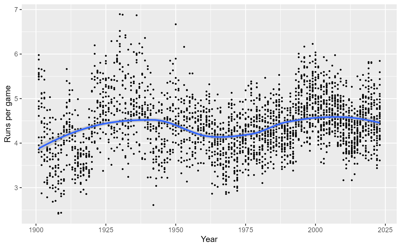
## Run scoring in the modern era by year
yrPlot("rpg", "Runs")
#> Warning: `aes_string()` was deprecated in ggplot2 3.0.0.
#> ℹ Please use tidy evaluation idioms with `aes()`.
#> ℹ See also `vignette("ggplot2-in-packages")` for more information.
#> `geom_smooth()` using formula = 'y ~ x'


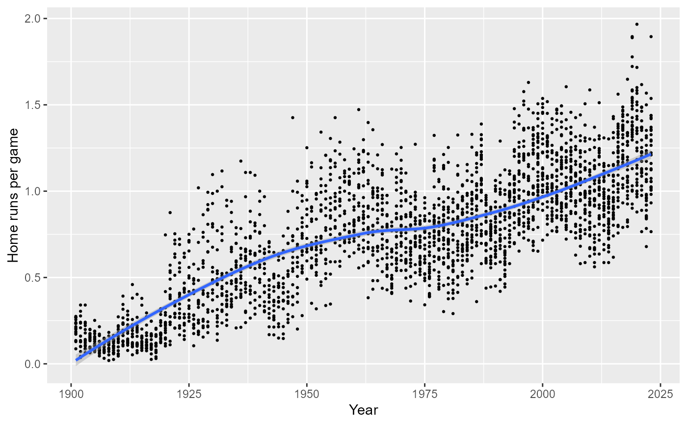
## Home runs per game by year
yrPlot("hrpg", "Home runs")
#> `geom_smooth()` using formula = 'y ~ x'


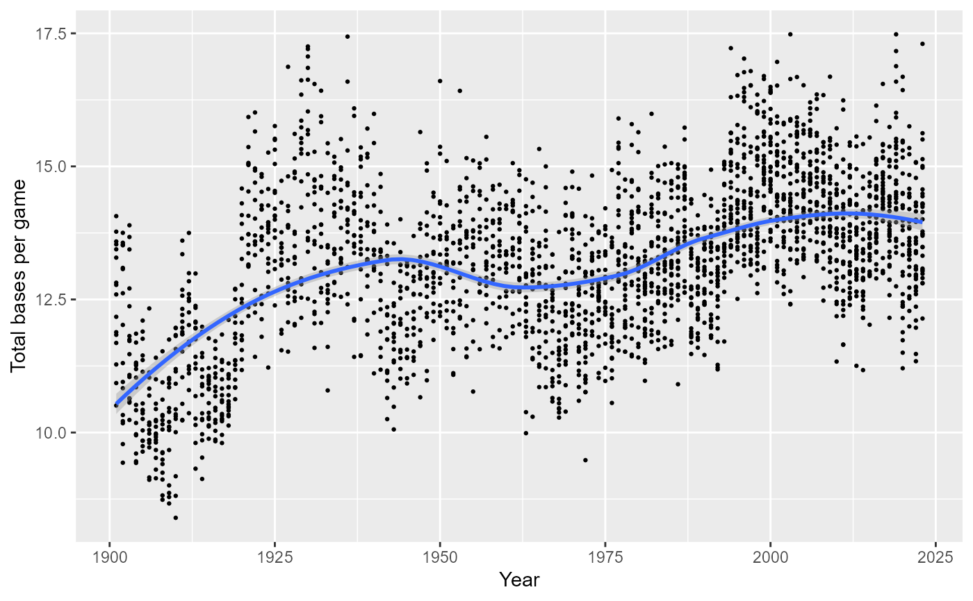
## Total bases per game by year
yrPlot("tbpg", "Total bases")
#> `geom_smooth()` using formula = 'y ~ x'


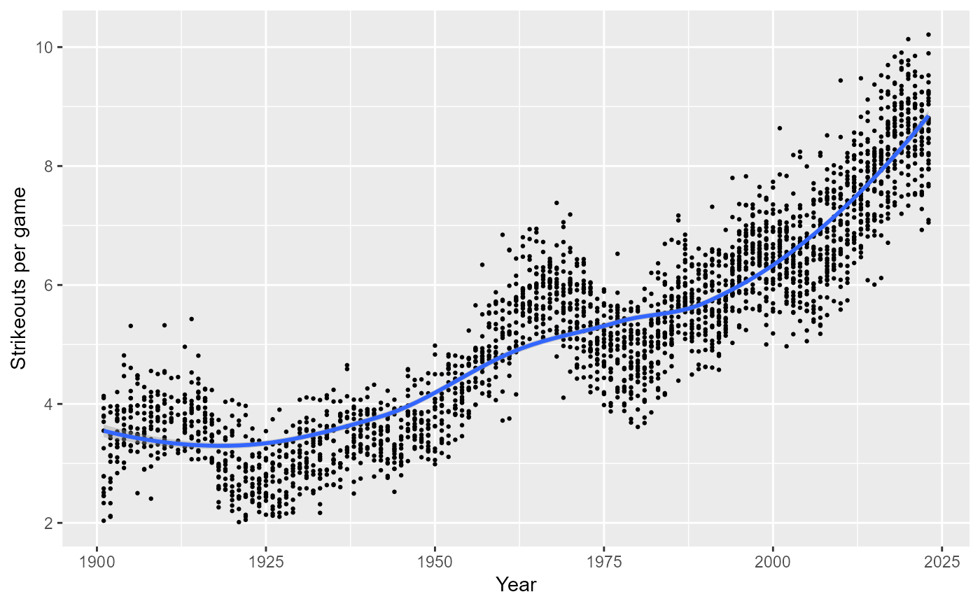
## Strikeouts per game by year
yrPlot("kpg", "Strikeouts")
#> `geom_smooth()` using formula = 'y ~ x'
#> Warning: Removed 16 rows containing non-finite outside the scale range
#> (`stat_smooth()`).
#> Warning: Removed 16 rows containing missing values or values outside the scale range
#> (`geom_point()`).


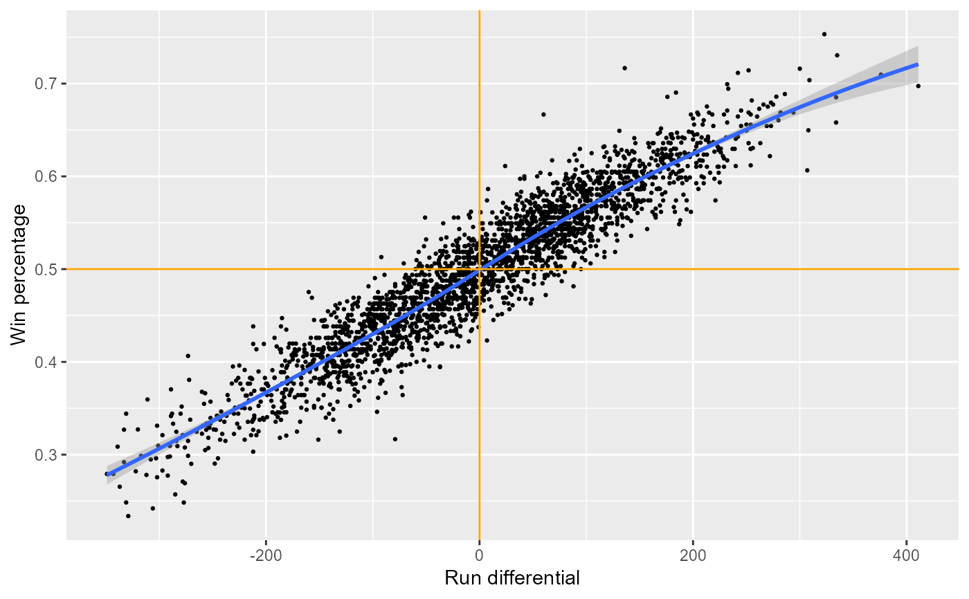
## Plot win percentage vs. run differential (R - RA)
ggplot(teams, aes(x = R - RA, y = WinPct)) +
   geom_point(size = 0.5) +
   geom_smooth(method="loess") + 
   geom_hline(yintercept = 0.5, color = "orange") +
   geom_vline(xintercept = 0, color = "orange") +
   labs(x = "Run differential", y = "Win percentage")
#> `geom_smooth()` using formula = 'y ~ x'


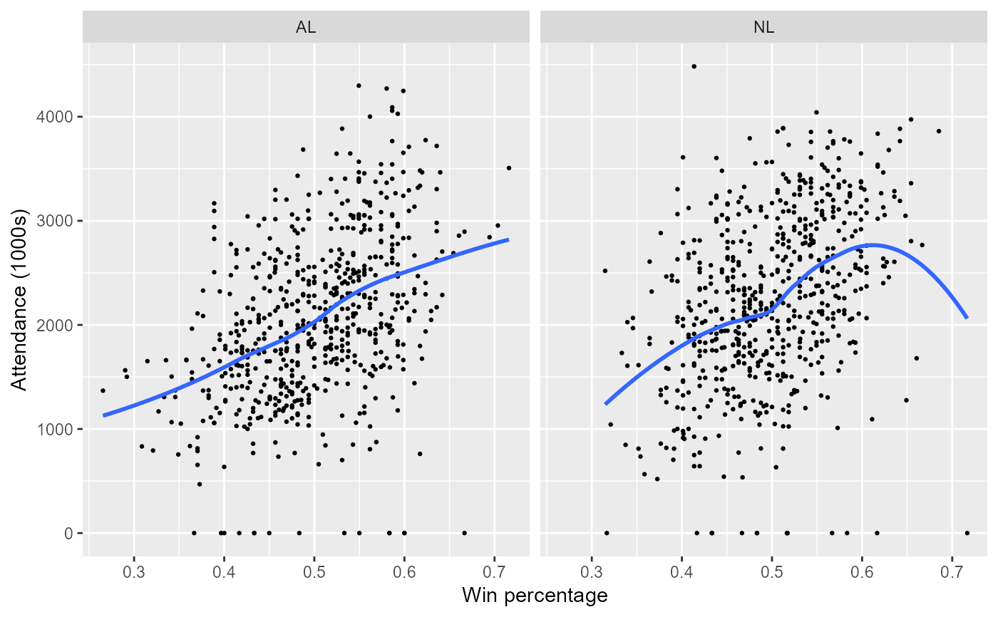
## Plot attendance vs. win percentage by league, post-1980
teams %>%  filter(yearID >= 1980) %>%
ggplot(., aes(x = WinPct, y = attendance/1000)) +
   geom_point(size = 0.5) +
   geom_smooth(method="loess", se = FALSE) +
   facet_wrap(~ lgID) +
   labs(x = "Win percentage", y = "Attendance (1000s)")
#> `geom_smooth()` using formula = 'y ~ x'


## Teams with over 4 million attendance in a season
teams %>% 
  filter(attendance >= 4e6) %>%
  select(yearID, lgID, teamID, Rank, attendance) %>%
  arrange(desc(attendance))
#> # A tibble: 9 × 5
#> # Groups:   yearID, teamID [9]
#>   yearID lgID  teamID  Rank attendance
#>    <int> <fct> <fct>  <int>      <int>
#> 1   1993 NL    COL        6    4483350
#> 2   2008 AL    NYA        3    4298655
#> 3   2007 AL    NYA        2    4271083
#> 4   2006 AL    NYA        1    4248067
#> 5   2005 AL    NYA        1    4090696
#> 6   1993 AL    TOR        1    4057947
#> 7   2008 NL    NYN        2    4042045
#> 8   1992 AL    TOR        1    4028318
#> 9   1991 AL    TOR        1    4001527

## Average season HRs by park, post-1980
teams %>% 
   filter(yearID >= 1980) %>%
   group_by(park) %>%
     summarise(meanHRpg = mean((HR + HRA)/Ghome), nyears = n()) %>%
     filter(nyears >= 10) %>%
     arrange(desc(meanHRpg)) %>%
     head(., 10)
#> # A tibble: 10 × 3
#>    park                        meanHRpg nyears
#>    <chr>                          <dbl>  <int>
#>  1 Yankee Stadium III              5.07     14
#>  2 The Ballpark at Arlington       4.87     11
#>  3 Great American Ball Park        4.81     20
#>  4 Rogers Centre                   4.77     18
#>  5 Angel Stadium of Anaheim        4.75     12
#>  6 Oriole Park at Camden Yards     4.70     32
#>  7 Coors Field                     4.63     29
#>  8 Target Field                    4.57     14
#>  9 Miller Park                     4.56     23
#> 10 Citizens Bank Park              4.56     20

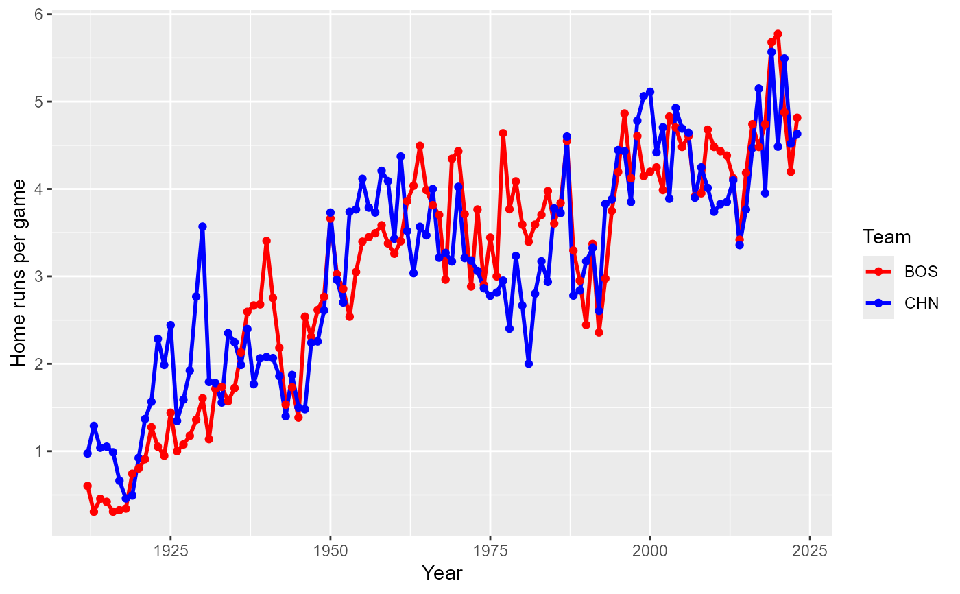
## Home runs per game at Fenway Park and Wrigley Field,
## the two oldest MLB parks, by year. Fenway opened in 1912.
teams %>% 
  filter(yearID >= 1912 & teamID %in% c("BOS", "CHN")) %>%
  mutate(hrpg = (HR + HRA)/Ghome) %>%
  ggplot(., aes(x = yearID, y = hrpg, color = teamID)) +
    geom_line(size = 1) +
    geom_point() +
    labs(x = "Year", y = "Home runs per game", color = "Team") +
    scale_color_manual(values = c("red", "blue"))


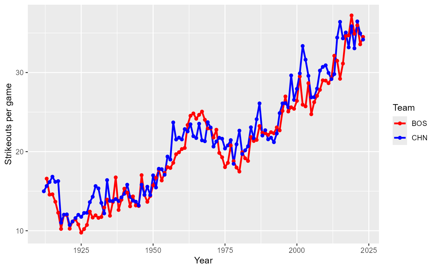
## Ditto for total strikeouts per game
teams %>% 
  filter(yearID >= 1912 & teamID %in% c("BOS", "CHN")) %>%
  mutate(kpg = (SO + SOA)/Ghome) %>%
  ggplot(., aes(x = yearID, y = kpg, color = teamID)) +
  geom_line(size = 1) +
  geom_point() +
  labs(x = "Year", y = "Strikeouts per game", color = "Team") +
  scale_color_manual(values = c("red", "blue"))  
#> Warning: Removed 1 row containing missing values or values outside the scale range
#> (`geom_line()`).
#> Warning: Removed 1 row containing missing values or values outside the scale range
#> (`geom_point()`).



if (FALSE) { # \dontrun{
if(require(googleVis)) {
motion1 <- gvisMotionChart(as.data.frame(teams), 
             idvar="teamID", timevar="yearID", chartid="gvisTeams",
             options=list(width=700, height=600))
plot(motion1)
#print(motion1, file="gvisTeams.html")

# Merge with avg salary for years where salary is available

teamsal <- Salaries %>%
                group_by(yearID, teamID) %>%
                summarise(Salary = sum(salary, na.rm = TRUE)) %>%
                select(yearID, teamID, Salary)

teamsSal <- teams %>%
                filter(yearID >= 1985) %>%
                left_join(teamsal, by = c("yearID", "teamID")) %>%
                select(yearID, teamID, attendance, Salary, WinPct) %>%
                as.data.frame(.)

motion2 <- gvisMotionChart(teamsSal, idvar="teamID", timevar="yearID",
  xvar="attendance", yvar="salary", sizevar="WinPct",
  chartid="gvisTeamsSal", options=list(width=700, height=600))
plot(motion2)
#print(motion2, file="gvisTeamsSal.html")

}
} # }