Team Payroll and the World Series
Michael Friendly
2025-09-08
Source:vignettes/payroll.Rmd
payroll.RmdThis vignette examines whether there is a relationship between total
team salaries (payroll) and World Series success. It was inspired by
Nolan & Lang (2015), “Baseball: Exploring Data in a Relational
Database”, Chapter 10 in Data
Science in R. They use SQL on the raw Lahman files
.csv, rather than the Lahman package.
Here, We largely use dplyr for data munging and
ggplot2 for plotting. In the process, we discover a few
errors in the data sets.
The data files
Start with loading the files we will use here. We do some pre-processing to make them more convenient for the analyses done later.
The Salaries data
The Salaries data.frame contains data on all players’
salaries from 1985-2016 in the latest release, v. 13.0.0, of the
Lahman package. (Additions to the Salaries
table in San Lahman’s database were discontinued after 2016.) We use the
sample_n function to display a random sample of
observations.
data("Salaries", package="Lahman")
str(Salaries)
## 'data.frame':    26428 obs. of  5 variables:
##  $ yearID  : int  2004 2007 2008 2009 2010 2011 2012 1986 1987 1988 ...
##  $ teamID  : Factor w/ 35 levels "ANA","ARI","ATL",..: 30 7 5 29 29 29 23 4 4 4 ...
##  $ lgID    : Factor w/ 2 levels "AL","NL": 2 1 1 1 1 1 1 1 1 1 ...
##  $ playerID: chr  "aardsda01" "aardsda01" "aardsda01" "aardsda01" ...
##  $ salary  : int  300000 387500 403250 419000 2750000 4500000 500000 600000 625000 675000 ...
sample_n(Salaries, 10)
##    yearID teamID lgID  playerID  salary
## 1    2004    MIL   NL  fordbe01  310000
## 2    2013    SFN   NL garcija01 4166667
## 3    2003    ATL   NL  fickro01 1000000
## 4    1997    SFN   NL gardnma01  900000
## 5    1993    NYN   NL thompry01  109000
## 6    1993    KCA   AL gubicma01 1250000
## 7    1999    KCA   AL appieke01 4800000
## 8    2009    LAN   NL mcdonja03  400750
## 9    1999    HOU   NL  holtch01  279000
## 10   2009    SDN   NL  baekch01  429900
The Teams data
The Teams data.frame contains a lot of information about
all teams that have ever played, with a separate observation for each
year. Here, we will mainly use this to get the team name
(team) from teamID and also to get the
information about World Series winners.
data("Teams", package="Lahman")
dim(Teams)
## [1] 3075   48
names(Teams)
##  [1] "yearID"         "lgID"           "teamID"         "franchID"
##  [5] "divID"          "Rank"           "G"              "Ghome"
##  [9] "W"              "L"              "DivWin"         "WCWin"
## [13] "LgWin"          "WSWin"          "R"              "AB"
## [17] "H"              "X2B"            "X3B"            "HR"
## [21] "BB"             "SO"             "SB"             "CS"
## [25] "HBP"            "SF"             "RA"             "ER"
## [29] "ERA"            "CG"             "SHO"            "SV"
## [33] "IPouts"         "HA"             "HRA"            "BBA"
## [37] "SOA"            "E"              "DP"             "FP"
## [41] "name"           "park"           "attendance"     "BPF"
## [45] "PPF"            "teamIDBR"       "teamIDlahman45" "teamIDretro"
We are only going to use the observations from 1985 on, and a few
variables, so we filter and select them now. Keep only the levels of
teamID in the data.
Teams <- Teams %>%
  select(yearID, lgID, teamID, name, divID, Rank, WSWin, attendance) %>%
  filter(yearID >= 1985) %>%
  mutate(teamID = droplevels(teamID))

sample_n(Teams, 10)
##    yearID lgID teamID              name divID Rank WSWin attendance
## 1    2005   AL    DET    Detroit Tigers     C    4     N    2024431
## 2    1993   AL    SEA  Seattle Mariners     W    4     N    2052638
## 3    2015   NL    ATL    Atlanta Braves     E    4     N    2001392
## 4    1993   NL    MON    Montreal Expos     E    2     N    1641437
## 5    2019   AL    NYA  New York Yankees     E    1     N    3304404
## 6    2003   AL    CLE Cleveland Indians     C    4     N    1730002
## 7    2009   AL    TOR Toronto Blue Jays     E    4     N    1876129
## 8    2017   NL    SDN  San Diego Padres     W    4     N    2138491
## 9    1987   NL    CIN   Cincinnati Reds     W    2     N    2185205
## 10   2021   AL    BOS    Boston Red Sox     E    2     N    1725323
The SeriesPost data
Post season records go back to 1884. There are 400 observations covering all aspects of post-season play.
data("SeriesPost", package="Lahman")
names(SeriesPost)
## [1] "yearID"       "round"        "teamIDwinner" "lgIDwinner"   "teamIDloser"
## [6] "lgIDloser"    "wins"         "losses"       "ties"
For each year, there are number of observations for the various levels of post-season play (Division titles, League titles, etc. A number of these designations have changed over the years, and I don’t know what they all mean.)
table(SeriesPost$round)
##
## AEDIV  ALCS ALDS1 ALDS2  ALWC ALWC1 ALWC2 ALWC3 ALWC4 AWDIV    CS NEDIV  NLCS
##     1    55    30    30     9     4     4     1     1     1     1     1    55
## NLDS1 NLDS2  NLWC NLWC1 NLWC2 NLWC3 NLWC4 NWDIV    WS
##    30    30     9     4     4     1     1     1   127
We are interested only in the World Series (WS), which
was first played in 1903. We filter for the years for which we have
salary data, and drop a couple of variables. The league IDs of the
winner and loser are factors, so we use droplevels to
include only the levels in recent history.
WS <- SeriesPost %>%
  filter(yearID >= 1985 & round == "WS") %>%
  select(-ties, -round) %>%
  mutate(lgIDloser = droplevels(lgIDloser),
         lgIDwinner = droplevels(lgIDwinner))
dim(WS)
## [1] 39  7
sample_n(WS, 6)
##   yearID teamIDwinner lgIDwinner teamIDloser lgIDloser wins losses
## 1   1988          LAN         NL         OAK        AL    4      1
## 2   2024          LAN         NL         NYA        AL    4      1
## 3   2006          SLN         NL         DET        AL    4      1
## 4   2005          CHA         AL         HOU        NL    4      0
## 5   1987          MIN         AL         SLN        NL    4      3
## 6   2016          CHN         NL         CLE        AL    4      3
A first look at Salaries
How many players do we have in each year?
table(Salaries$yearID)
##
## 1985 1986 1987 1988 1989 1990 1991 1992 1993 1994 1995 1996 1997 1998 1999 2000
##  550  738  627  663  711  867  685  769  923  884  986  931  925  998 1006  836
## 2001 2002 2003 2004 2005 2006 2007 2008 2009 2010 2011 2012 2013 2014 2015 2016
##  860  846  827  831  831  819  842  856  813  830  839  848  815  802  817  853
What is the range of salaries, across all years?
range(Salaries$salary)
## [1]        0 33000000
And, year by year?
Salaries %>%
  group_by(yearID) %>%
  summarise(min=min(salary),
            max=max(salary))
## # A tibble: 32 × 3
##    yearID    min     max
##     <int>  <int>   <int>
##  1   1985  60000 2130300
##  2   1986  60000 2800000
##  3   1987  62500 2127333
##  4   1988  62500 2340000
##  5   1989  62500 2766667
##  6   1990 100000 3200000
##  7   1991 100000 3800000
##  8   1992 109000 6100000
##  9   1993      0 6200000
## 10   1994  50000 6300000
## # ℹ 22 more rows
Hmm, there is a salary==0 in 1993, maybe there are
others.
which(Salaries$salary==0)
## [1] 11609 14751
Who are they? (We could also look up their playerIDs in
Lahman::People.)
Salaries[which(Salaries$salary==0),]
##       yearID teamID lgID  playerID salary
## 11609   1993    NYA   AL jamesdi01      0
## 14751   1999    PIT   NL martija02      0
These must be errors. Get rid of them. Reminder: Check further; maybe file an issue in the Lahman package!
Get team payrolls
We want to sum the salary for each team for each year.
We might as well make it in millions. All those zeros hurt my eyes.
payroll <- Salaries %>%
                group_by(teamID, yearID) %>%
                summarise(payroll = sum(salary)/1000000)
head(payroll)
## # A tibble: 6 × 3
## # Groups:   teamID [1]
##   teamID yearID payroll
##   <fct>   <int>   <dbl>
## 1 ANA      1997    31.1
## 2 ANA      1998    41.3
## 3 ANA      1999    55.4
## 4 ANA      2000    51.5
## 5 ANA      2001    47.5
## 6 ANA      2002    61.7
Merge team names into payroll
It will be more convenient to have the team names included in the
payroll data.frame. The Teams data frame also
contains the Y/N indicator WSWin for World
Series winners, so we might as well include this too.
payroll <- merge(payroll, Teams[,c("yearID", "teamID","name", "WSWin")],
                 by=c("yearID", "teamID"))
sample_n(payroll, 10)
##    yearID teamID payroll                          name WSWin
## 1    2006    MIN   63.40               Minnesota Twins     N
## 2    2007    MIL   70.99             Milwaukee Brewers     N
## 3    2016    LAA  137.25 Los Angeles Angels of Anaheim     N
## 4    2005    OAK   55.43             Oakland Athletics     N
## 5    2003    FLO   49.45               Florida Marlins     Y
## 6    2009    COL   75.20              Colorado Rockies     N
## 7    2000    MIL   36.51             Milwaukee Brewers     N
## 8    1999    ANA   55.39                Anaheim Angels     N
## 9    2013    NYA  231.98              New York Yankees     N
## 10   1989    CAL   15.10             California Angels     N
Note that we could also do this using left_join in the
dplyr package. There is probably a more tidy
way to subset the variables from the Teams data set than
using Teams[, c()], but, hey– this works.
left_join(payroll, Teams[,c("yearID", "teamID","name", "WSWin")],
          by=c("yearID", "teamID")) %>%
  sample_n(10)
WSWin is a character variable. Convert it to a
factor.
Check the values:
table(payroll$WSWin, useNA="ifany")
##
##    N    Y <NA>
##  859   31   28
There is something wrong here! There shouldn’t be any
NAs. We leave this for further study, and another
Reminder to file an issue if we figure out what the
problem is.
Boxplots of payroll
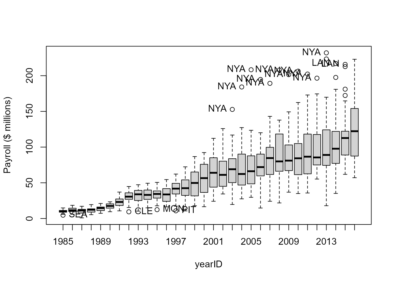
Let’s look at the distributions of payroll by year. The observations are teams.
boxplot(payroll ~ yearID, data=payroll, ylab="Payroll ($ millions)") What are the outliers? Are there any teams that crop up repeatedly?
car::Boxplot makes this easy, and also returns the labels
of the outliers. We don’t load the car package, because
car also contains a Salary dataset.
out <- car::Boxplot(payroll ~ yearID, data=payroll,
             id=list(n=1,
                     labels=as.character(payroll$teamID)),
             ylab="Payroll ($ millions)")
Most of the outliers are the New York Yankees (NYA):
table(out)
## out
## CLE LAN MON NYA PIT SEA
##   1   2   1  11   1   1
Payroll has obviously increased dramatically over time. So has the
variability across teams. For any modelling, we would probably want to
use \log(payroll). We might also want to look separately at
the American and National leagues.
Correcting for inflation
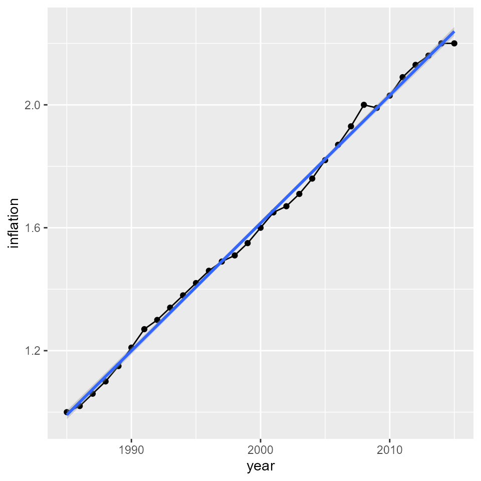
For proper comparisons, we should correct for inflation. Lets do this by scaling salary back to 1985 dollars, The data below gives inflation rates for all subsequent years. It comes from Nolan & Lang, extended to 2015 using (https://www.in2013dollars.com/).
inflation = c(1,    1.02, 1.06, 1.10, 1.15, 1.21,
              1.27, 1.30, 1.34, 1.38, 1.42, 1.46, 1.49, 1.51, 1.55, 1.60,
              1.65, 1.67, 1.71, 1.76, 1.82, 1.87, 1.93, 2.00, 1.99, 2.03,
              2.09, 2.13, 2.16, 2.20, 2.20 )

inflation.df <- data.frame(year=1985:2015, inflation)

# plot inflation rate
ggplot(inflation.df, aes(y=inflation, x=year)) +
  geom_point() +
  geom_line() +
  geom_smooth(method="lm")
This is close enough to linear, that we could use the linear
regression predicted value as a simple computation of the inflation
rate. (A better way, of course, would be to use the actual inflation
rate; this would entail merging payroll with
inflation.df by year, and doing the computation.)
infl.lm <- lm(inflation ~ year, data=inflation.df)
(coefs <- coef(infl.lm))
## (Intercept)        year
##   -81.57032     0.04159
Scale payroll by dividing by linear prediction of
inflation rate, producing payrollStd.
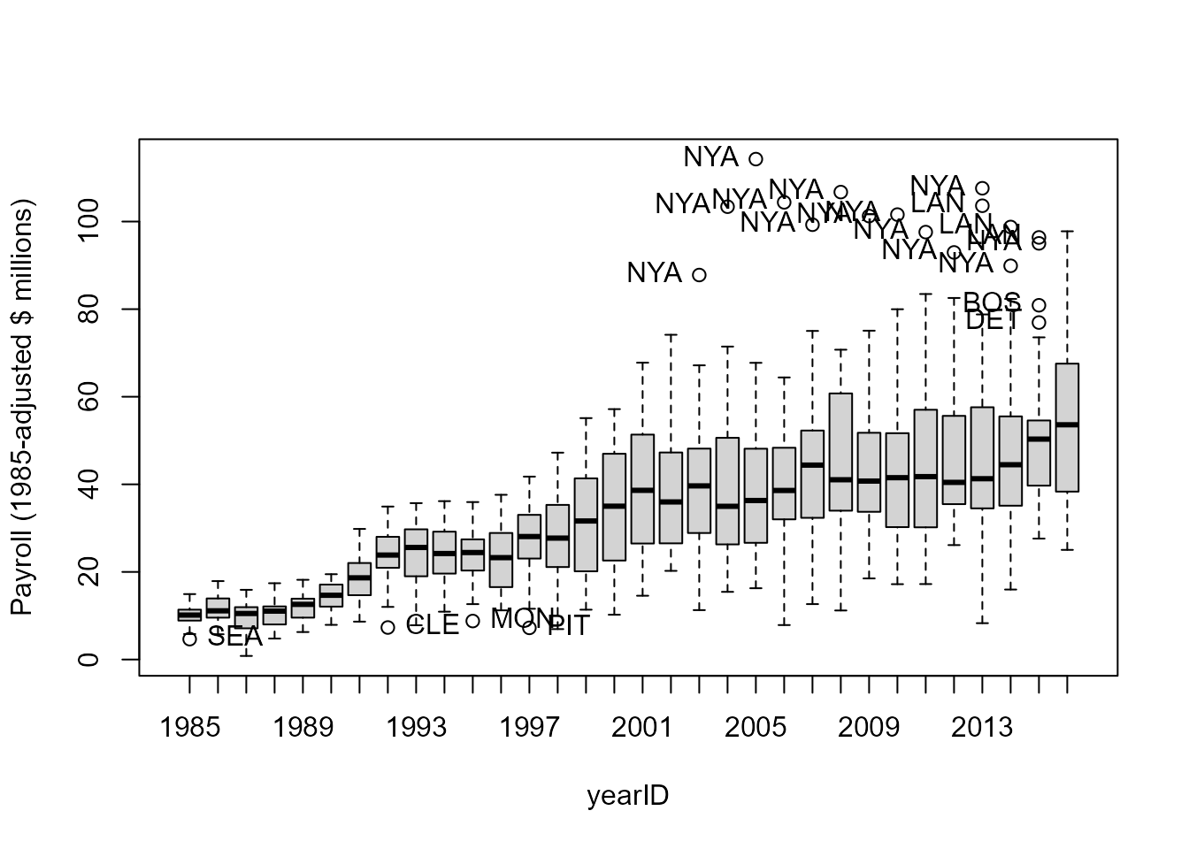
Boxplot again, of inflation-adjusted payroll. The increase after 2000 doesn’t seem so large.
car::Boxplot(payrollStd ~ yearID, data=payroll,
             id = list(labels=as.character(payroll$teamID)),
             ylab="Payroll (1985-adjusted $ millions)")
##  [1] "SEA" "CLE" "MON" "PIT" "NYA" "NYA" "NYA" "NYA" "NYA" "NYA" "NYA" "NYA"
## [13] "NYA" "NYA" "LAN" "NYA" "LAN" "NYA" "BOS" "DET" "LAN" "NYA"
Salaries of World Series winning teams
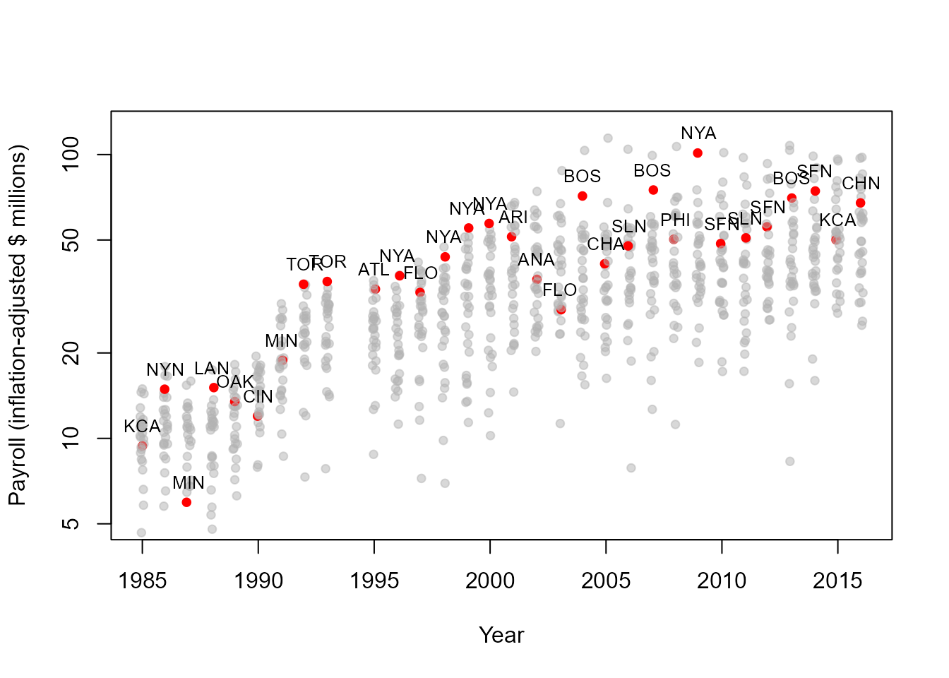
To what extent are the World Series winners those among the highest in payroll? A simple way to look at this is to plot the team payrolls across years, and mark the World Series winner for each year.
This plot shows inflation-adjusted payroll on a log scale to avoid the dominating influence of the most recent years. We jitter the points to avoid overplotting, and use a transparent gray color for the non-winners, red for the winner in each year.
Cols <- ifelse(payroll$WSWin=='Y', "red", gray(.7, alpha=0.5))
with(payroll, {
  plot(payrollStd ~ jitter(yearID, 0.5),
       ylab = "Payroll (inflation-adjusted $ millions)",
       ylim = c(5,125), log = "y",
       xlab = "Year",
       pch = 19, cex = 0.8, col = Cols)
})
with(payroll[payroll$WSWin == 'Y',],
     text(y = payrollStd, x = yearID, labels = teamID, pos = 3, cex = 0.8) )
By and large, the World Series winners tend to be in the upper portion of the payrolls for each year.
Further analyses: Your turn
Here are some questions to provoke further analyses of these data sets. If you find something interesting, post it in a Github Gist or forward it to Team Lahman as in a Lahman issue.
Our boxplots used total payroll in millions. Would the plots be clearer if we plotted payroll on a log scale?
Follow-up the suggestion to fit a linear model predicting
log(payroll)from some of the available predictors.Examine the trend of team salaries over time for World Series losers. Does it look the same or different than that for the winning teams?
What kind of analysis would you do to address this statement: “For teams that make it to the World series, the one with the larger payroll is more likely to win.”
Is there any relationship between the number of team wins in a season and winning the World series?