Salaries table
Salaries.RdPlayer salary data.
Usage
data(Salaries)Format
A data frame with 26428 observations on the following 5 variables.
yearIDYear
teamIDTeam; a factor
lgIDLeague; a factor
playerIDPlayer ID code
salarySalary
Source
Lahman, S. (2026) Lahman's Baseball Database, 1871-2025, 2026 version, https://sabr.org/lahman-database/
Examples
# what years are included?
summary(Salaries$yearID)
#>    Min. 1st Qu.  Median    Mean 3rd Qu.    Max.
#>    1985    1994    2001    2001    2009    2016

# how many players included each year?
table(Salaries$yearID)
#>
#> 1985 1986 1987 1988 1989 1990 1991 1992 1993 1994 1995 1996 1997 1998 1999 2000
#>  550  738  627  663  711  867  685  769  923  884  986  931  925  998 1006  836
#> 2001 2002 2003 2004 2005 2006 2007 2008 2009 2010 2011 2012 2013 2014 2015 2016
#>  860  846  827  831  831  819  842  856  813  830  839  848  815  802  817  853

# Team salary data

require("dplyr")
require("ggplot2")

# Total team salaries by league, team and year
teamSalaries <- Salaries %>%
                  group_by(lgID, teamID, yearID) %>%
                  summarise(Salary = sum(as.numeric(salary))) %>%
                  group_by(yearID, lgID) %>%
                  arrange(desc(Salary))
#> `summarise()` has grouped output by 'lgID', 'teamID'. You can override using
#> the `.groups` argument.

#######################################
# Highest paid players each year:
maxSal <- Salaries %>%
            group_by(yearID) %>%
            filter(salary == max(salary))
maxPlayers <- bind_rows(lapply(maxSal$playerID, playerInfo)) %>%
                  select(-playerID)
maxSal <- bind_cols(maxPlayers, maxSal)

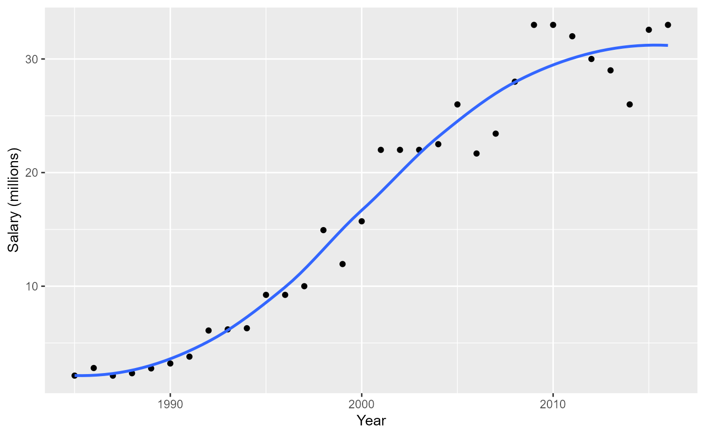
# Plot maximum MLB salary by year (1985-present)
ggplot(maxSal, aes(x = yearID, y = salary/1e6)) +
   geom_point() +
   geom_smooth(se = FALSE) +
   labs(x = "Year", y = "Salary (millions)")
#> `geom_smooth()` using method = 'loess' and formula = 'y ~ x'


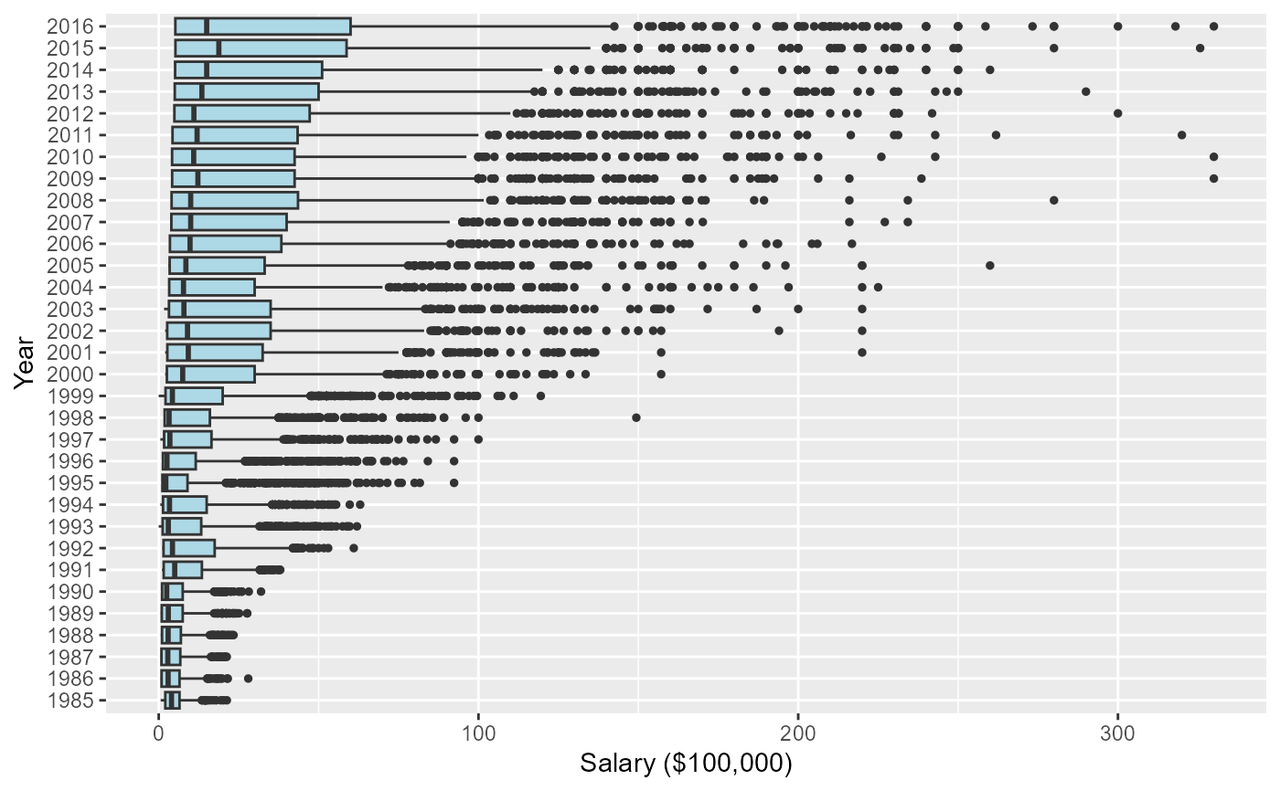
# Plot salary distributions by year for all players
ggplot(Salaries, aes(x = factor(yearID), y = salary/1e5)) +
   geom_boxplot(fill = "lightblue", outlier.size = 1) +
   labs(x = "Year", y = "Salary ($100,000)") +
   coord_flip()


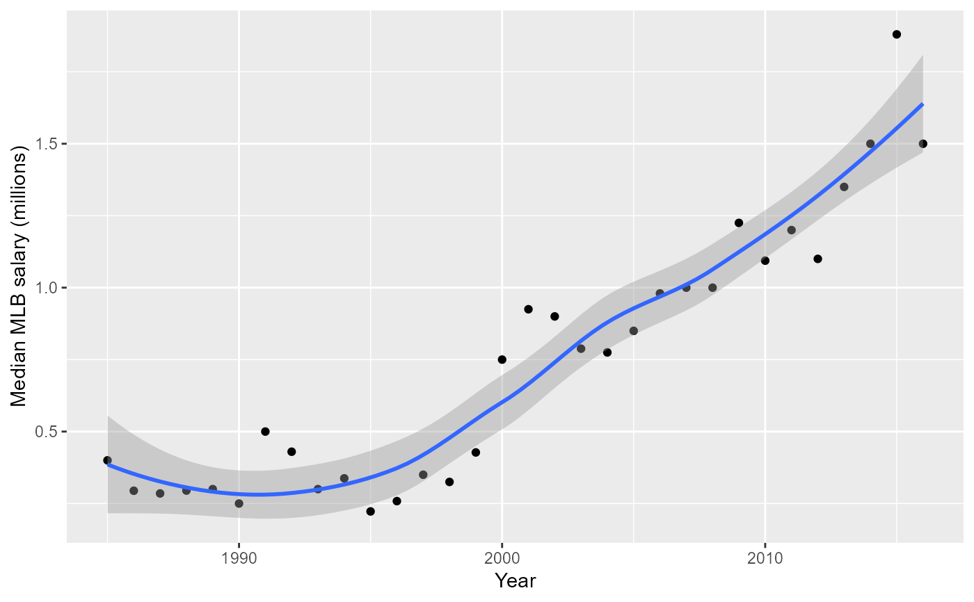
# Plot median MLB salary per year
Salaries %>%
   group_by(yearID) %>%
   summarise(medsal = median(salary)) %>%
   ggplot(., aes(x = yearID, y = medsal/1e6)) +
   geom_point() +
   geom_smooth() +
   labs(x = "Year", y = "Median MLB salary (millions)")
#> `geom_smooth()` using method = 'loess' and formula = 'y ~ x'


# add salary to Batting data
batting <- Batting %>%
              filter(yearID >= 1985) %>%
              left_join(select(Salaries, playerID, yearID, teamID, salary),
                         by=c("playerID", "yearID", "teamID"))
str(batting)
#> 'data.frame':	53195 obs. of  23 variables:
#>  $ playerID: chr  "aardsda01" "aardsda01" "aardsda01" "aardsda01" ...
#>  $ yearID  : int  2004 2006 2007 2008 2009 2010 2012 2013 2015 1985 ...
#>  $ stint   : int  1 1 1 1 1 1 1 1 1 1 ...
#>  $ teamID  : Factor w/ 149 levels "ALT","ANA","ARI",..: 117 35 33 16 116 116 93 94 4 5 ...
#>  $ lgID    : Factor w/ 7 levels "AA","AL","FL",..: 5 5 2 2 2 2 2 5 5 2 ...
#>  $ G       : int  11 45 25 47 73 53 1 43 33 54 ...
#>  $ AB      : int  0 2 0 1 0 0 0 0 1 0 ...
#>  $ R       : int  0 0 0 0 0 0 0 0 0 0 ...
#>  $ H       : int  0 0 0 0 0 0 0 0 0 0 ...
#>  $ X2B     : int  0 0 0 0 0 0 0 0 0 0 ...
#>  $ X3B     : int  0 0 0 0 0 0 0 0 0 0 ...
#>  $ HR      : int  0 0 0 0 0 0 0 0 0 0 ...
#>  $ RBI     : int  0 0 0 0 0 0 0 0 0 0 ...
#>  $ SB      : int  0 0 0 0 0 0 0 0 0 0 ...
#>  $ CS      : int  0 0 0 0 0 0 0 0 0 0 ...
#>  $ BB      : int  0 0 0 0 0 0 0 0 0 0 ...
#>  $ SO      : int  0 0 0 1 0 0 0 0 1 0 ...
#>  $ IBB     : int  0 0 0 0 0 0 0 0 0 0 ...
#>  $ HBP     : int  0 0 0 0 0 0 0 0 0 0 ...
#>  $ SH      : int  0 1 0 0 0 0 0 0 0 0 ...
#>  $ SF      : int  0 0 0 0 0 0 0 0 0 0 ...
#>  $ GIDP    : int  0 0 0 0 0 0 0 0 0 0 ...
#>  $ salary  : int  300000 NA 387500 403250 419000 2750000 500000 NA NA NA ...

#######################################
# Average salaries by teams, over years
#######################################

# Some franchises are multiply named, so add a new variable
# 'franchise' to the Salaries data as a lookup table

franchise <- c(`ANA` = "LAA", `ARI` = "ARI", `ATL` = "ATL",
               `BAL` = "BAL", `BOS` = "BOS", `CAL` = "LAA",
               `CHA` = "CHA", `CHN` = "CHN", `CIN` = "CIN",
               `CLE` = "CLE", `COL` = "COL", `DET` = "DET",
               `FLO` = "MIA", `HOU` = "HOU", `KCA` = "KCA",
               `LAA` = "LAA", `LAN` = "LAN", `MIA` = "MIA",
               `MIL` = "MIL", `MIN` = "MIN", `ML4` = "MIL",
               `MON` = "WAS", `NYA` = "NYA", `NYM` = "NYN",
               `NYN` = "NYN", `OAK` = "OAK", `PHI` = "PHI",
               `PIT` = "PIT", `SDN` = "SDN", `SEA` = "SEA",
               `SFG` = "SFN", `SFN` = "SFN", `SLN` = "SLN",
               `TBA` = "TBA", `TEX` = "TEX", `TOR` = "TOR",
               `WAS` = "WAS")

Salaries$franchise <- unname(franchise[Salaries$teamID])

# Average salaries annual salaries by team, in millions USD
avg_team_salaries <- Salaries %>%
    group_by(yearID, franchise, lgID) %>%
    summarise(salary= mean(salary)/1e6) %>%
    filter(!(franchise == "CLE" & lgID == "NL"))
#> `summarise()` has grouped output by 'yearID', 'franchise'. You can override
#> using the `.groups` argument.

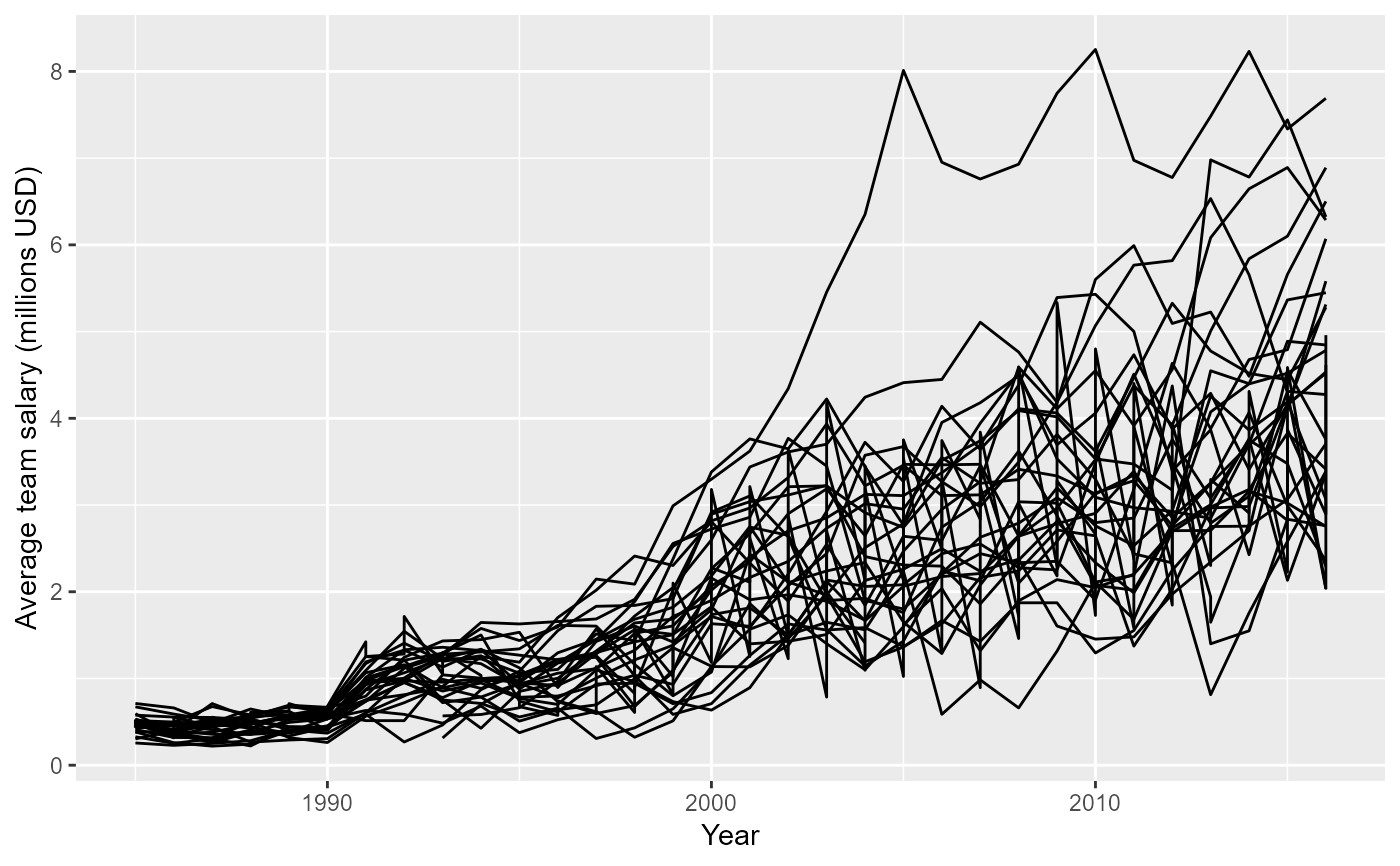
# Spaghetti plot of team salary over time by team
# Yankees have largest average team salary since 2003
ggplot(avg_team_salaries,
       aes(x = yearID, y = salary, group = factor(franchise))) +
       geom_path() +
       labs(x = "Year", y = "Average team salary (millions USD)")
